Land Cover Change Classification (Training, Testing and Selection)
As the steps of both 2020 and 2022 are similar, the images and descriptions seen below are repeated.
SCP Tool will allow us to input training and testing data as ROI and Signature for the SCP tool to perform Classification.
Summary of Methodology
Training
1. Land Cover Types
2. Fine tuning using Standard Deviation (S.D)
3. Evaluation of algorithms using Spectral Distance
4. Run SCP Classification on 2 Algorithm: Minimum Distance and Maximum Likelihood
Testing
1. Add testing samples for each land cover type
2. Calculate accuracy for both algorithms using the same test samples in previous step
3. Select better Algorithm
4. Retrain samples for those accuracy and PA less than 75%
Final evaluation of classification model
Training
1. Land Cover Types
The Land Cover Types (MC ID) we determine are:
a. Vegetation
b. Water body
c. Buildings
d. Bare land
e. Impervious surfaces
f. Cloud
g. Cloud shadow
For [a, b, c, d, e] there will 10 samples each. For [f, g] there will be 5 each.
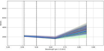
2. Fine tuning using Standard Deviation (S.D)
Those S.D of the Wavelength determined by the SCP Tool which are too far from most of them will be deleted and another sample will be chosen. An example below shows a decent sample with low S.D among the samples.
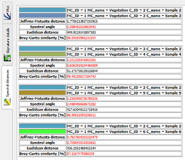
3. Evaluation of algorithms using Spectral Distance
Screenshot of Sample Data being added
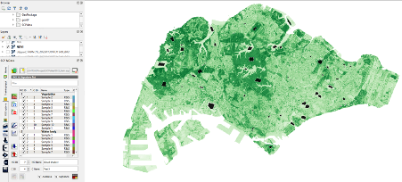
With all the ROI added into Training data, the spectral distance can be calculated.
Based on the Spectral distance, it is highly likely that the Minimum Distance algorithm will be good. This is because most of the Euclidean Distance are within the acceptable range across all Types, as compared to the other metrics.
An example of the entire results is shown below.
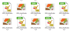
4. Run SCP Classification on 2 Algorithm: Minimum Distance and Maximum Likelihood
The SCP would produce an output for each Algorithm which is in GeoTiff format.
Results and output of Selected Classification will be shown below.
Testing
1. Add testing samples for each land cover type
This test sample will be used for accuracy calculation. The same test sample will be used on both algorithms to see which performs better in general.
For each Land Cover Type, there will be 3 Samples. We are performing the 70-30 rule for analytics in general.
None of the testing samples will not be the same as the training input.
2. Calculate accuracy for both algorithm using the same test samples in previous step
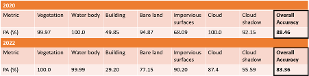
We obtain the results of the Overall Accuracy and [PA] from the confusion matrix for each of the algorithms at this step.
3. Selection of algorithm
True enough, based on the spectral distances, the Minimum Distance Algorithm classified better than the Maximum Likelihood Algorithm in terms of Overall and [PA].
Therefore, Minimum Distance Algorithm is selected for further improvement.
4. Retraining for PA less than 75%
Across both Study years of 2020 and 2022, the major issue is the classification of buildings. It has poor classification PA of 40% and 20% respectively. The other classification issue is for cloud shadow with PA of 45% and 35% respectively.
However, the main concern is the buildings as compared to cloud cover. This is because for buildings, it has some classified as vegetation which will affect the analysis of land cover change. Another minor misclassification would be buildings being classified as Impervious Surfaces.
Thus, the goal is to reiterate the Training Sample up to 10 times and choose the best training model base on Overall Accuracy and [PA] for each land cover type.
Sample of Iterations “put into action”
Final evaluation of classification model
During the iteration and retraining of sample data, we noticed that the more diverse we try to classify each land type, the worse the classification becomes. For example, the sunlight is different around Tuas Area which makes buildings brighter and then classified as bare land. And in areas which are darker, it classified buildings as vegetation and water bodies.
Despite 10 iterations of training samples, buildings are still poorly classified. However, most of these misclassifications classify buildings as other urban features. If we create a more generic category of ‘urban’ features, the effects of this misclassification is mitigated.
Generic Categorizations:
- [Vegetation (1), Waterbody (2)] = Natural
- [Buildings (3), Bar land (4), Impervious surface (5)] = Urbanisation
- [Cloud (6), Cloud shadow (7)] = Clouds
The raster which was produced for the selected iteration is saved as a Geo Tiff File to be used for the next task.
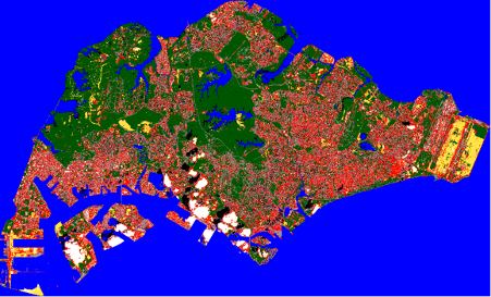
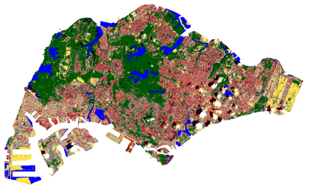
Output of Classification
2020:
2022:
Data Analysis (Land Cover Change)
Summary of Methodology
1. Change Detection Processing
a. Generation of Change Detection Map
b. Selection of interested bands
2. Data Cleaning
3. Area Calculation
1. Change Detection Processing
a. Generation of Change Detection Map
Using the Classification Output selected above for 2020 and 2022, we can input these layers into SCP Change Detection Tool.
The Tool will compare for each land cover type and extract the changes. Since we have 7 types of classification, we will have 49 Classes of change.
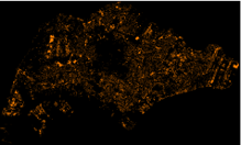
Below shows the initial output of the land cover change.
However, this initial output has no significant meaning.
b. Selection of Interested Bands
To make the output more meaningful, we need to select the bands we are interested in. In this case we plan to see the [1] Vegetation converting to Urban and [2] Urban being Converted to Vegetation between 2020 – 2022.
The Tool also produces a matrix table which we can use to determine the interest bands.
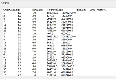
We select the Cross Class Code based on the New Class and Reference Class. The Cross Class Code selection are as follows:
Forest to Urban (Orange)– 6, 10, 15
Urban to Forest (Green) – 4, 7, 11
With this we can generate 2 layers with the results.
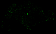
Forest to Urban (Initial Output)
Urban to Forest (Initial Output)
However, as it is based on classification which is not 100% accurate, we need to clean the data.
2. Data Cleaning
A tedious and manual task is done to ensure that the data is clean. We draw a grid and compare the original TCC/FCC of 2020 and 2022 to see if each part which is highlighted above is correct. We do this for all grids and only keep the changes that are accurate.
Example of Cleaning Process Grid
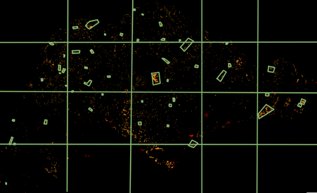
After selecting using hand drawn polygons, we simply clip the raster layer.
3. Area Calculation
Using the “Raster Layer Unique Values Report” in GIS Toolbox to calculate the area via pixels and their classification.
However, as the results returned gave the area of all “Cross Class Code”, we will again use those we have chosen to be used for the Area Calculation.
With that, we are able to Sum the Area of Forested Areas converted to Urbanisation as well as the Sum of Area of Urbanisation being brought back to Vegetation.
The final results of area calculation and the output of the cleaned layer can be found here.
Data Analysis (Land Surface Temperature)
Summary of Methodology
1. Generation of LST Map using Google Earth Engine
2. Export raster layer as GeoTiff
3. Average temperature change calculation
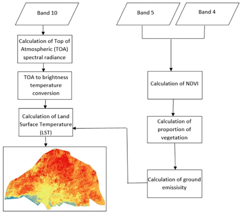
Using the formula to derive the LST found online, the main bands that were useful for the analysis are band 4, 5 and 10 respectively.
1. Generation of LST Map using Google Earth Engine
Using Google Earth Engine, the code snippet below are the JavaScript code and functions used to render the LST across the main island of Singapore.
In summary the process will first search all available Landsat 8 collection 2, tier 1 level 2 satellite images within the defined periods. A cloud masking function is defined to filter out pixels that have clouds or cloud shadows and the the average LST is aggregated at the pixel granularity with the appropriate function to apply scale factors for deriving the LST in Celsius.
// Assign a variable to filter the day of year from Jan 1 to Dec 31
var DATE_RANGE = ee.Filter.dayOfYear(1, 360);
// Assign a variable to filter years from 2018-2020 or 2020-2022
var YEAR_RANGE = ee.Filter.calendarRange(2020, 2022, 'year');
// Assign a variable to delineate the area of interest
// Create you own aoi polygon using the Geometry tools in the map window.
// Rename you geometry to match the assigned variable name
var STUDYBOUNDS = aoi;
// Assign a variable to display images in the map window
var DISPLAY = true;
// Set the base-map to display as satellite
Map.setOptions("SATELLITE");
// Assign a variable to the sensor-specific bands unique to each Landsat mission.
var LC08_bands = ["ST_B10", "QA_PIXEL"]; // Landsat 8 surface temperature (ST) & QA_Pixel bands
// To mask clouds and cloud shadows based on the QA_PIXEL band of Landsat 8 & 9
// Information on bit values for the QA_PIXEL band refer to:
// https://developers.google.com/earth-engine/datasets/catalog/LANDSAT_LC08_C02_T1_L2#bands
function cloudMask(image){
var qa = image.select("QA_PIXEL");
var mask = qa.bitwiseAnd(1 << 3).or(qa.bitwiseAnd(1 << 4));
return image.updateMask(mask.not());
}
// Assign variables to import the Landsat Collection 2, Tier 1, Level 2 image collections, selecting the ST and QA_PIXEL bands, and spatially filtering the image collection by the aoi
var L8 = ee.ImageCollection('LANDSAT/LC08/C02/T1_L2')
.select("ST_B10", "QA_PIXEL")
.filterBounds(STUDYBOUNDS)
.filter(DATE_RANGE)
.filter(YEAR_RANGE)
.map(cloudMask);
// Filter the collection by the CLOUD_COVER property so each image contains less than 100% cloud cover
var filtered_L8 = L8.filter(ee.Filter.lt("CLOUD_COVER", 100));
// Function using Landsat scale factors for deriving ST in Kelvin and Celsius
function applyScaleFactors(image){
var thermalBands = image.select("ST_B10")
.multiply(0.00341802)
.add(149.0)
.subtract(273.15);
return image.addBands(thermalBands, null, true);
}
// Define a variable to apply scale factors to the filtered image collection
var landsatST = filtered_L8.map(applyScaleFactors);
// Define a variable to calculate mean ST for each pixel
// throughout the filtered image collection
var mean_LandsatST = landsatST.mean();
// Define a variable to use the clip function to subset the imagery to the aoi
var clip_mean_ST = mean_LandsatST.clip(STUDYBOUNDS);
// Add the image to the map window, defining min/max values, a palette
// for symbology, assign a name to the visualization, and display the result
Map.addLayer(clip_mean_ST, {
bands : "ST_B10",
min: 28, max : 47,
palette: ['blue', 'white', 'red']
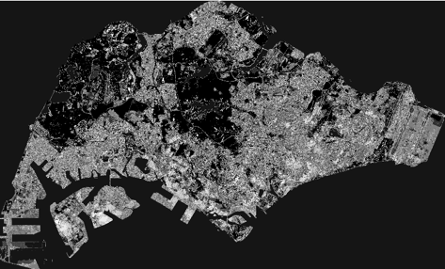
}, "ST", DISPLAY);Below shows a sample output generated from the above code snippet. 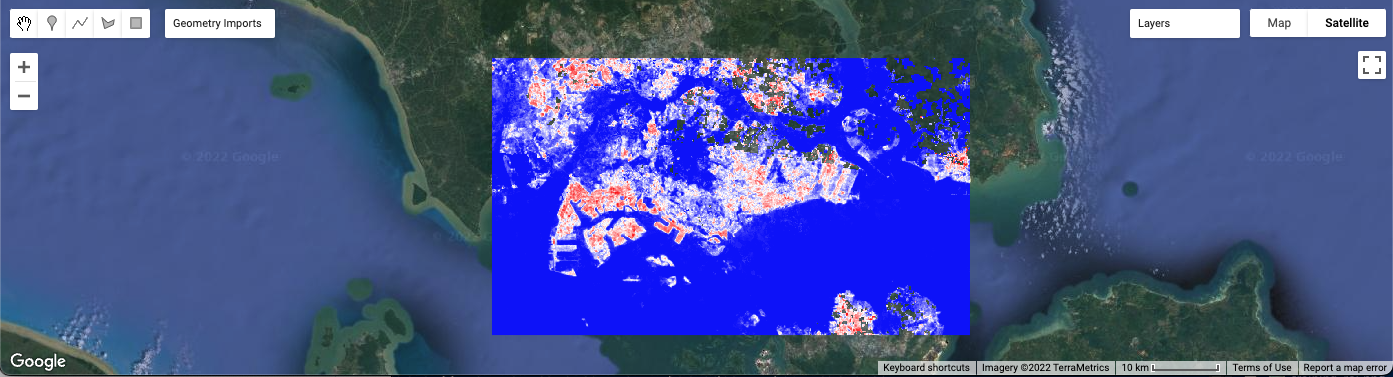
2. Export raster layer as GeoTiff
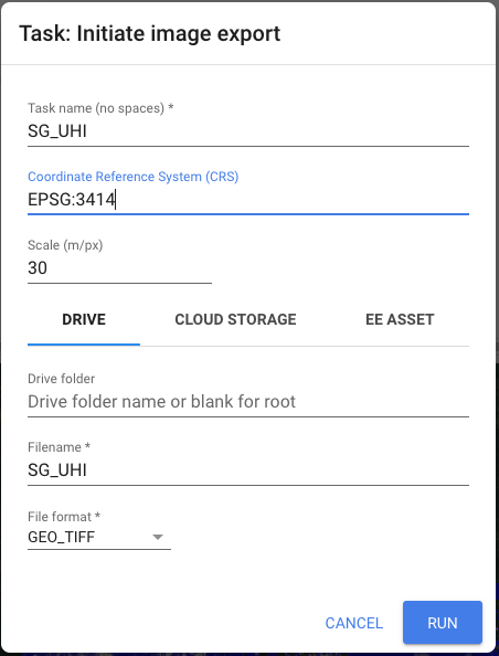
The code snippet below provides the function to export the LST raster layer in GeoTiff format into Google Drive which then can be imported into QGIS for further data processing and visualization.
Export.image.toDrive({
  image: clip_mean_ST,
  description: "SG_UHI",
  scale: 30,
  region: aoi
})
Under the Tasks tab, an unsubmitted task will be queued and running it will display a popup to confirm the file name, coordinate reference system, file format and save location
3. Average temperature change calculation
Using the LST rasters generated from 2018 to 2020 and 2020 to 2022 respectively, the average temperature difference between the two periods can be calculated at the planning area level by first clipping the raster layer only to the main island of Singapore using the Clip Raster by Mask Layer function.
Using the 2019 subzone area data from data.gov, the first step is to dissolve the subzone by planning area followed by getting the minimum, maximum and average raster values by planning area can be derived by using the Zonal statistics function found in the Toolbox. (Toolbox > Raster analysis > Zonal statistics)
Below is the sample inputs for the Zonal statistics function 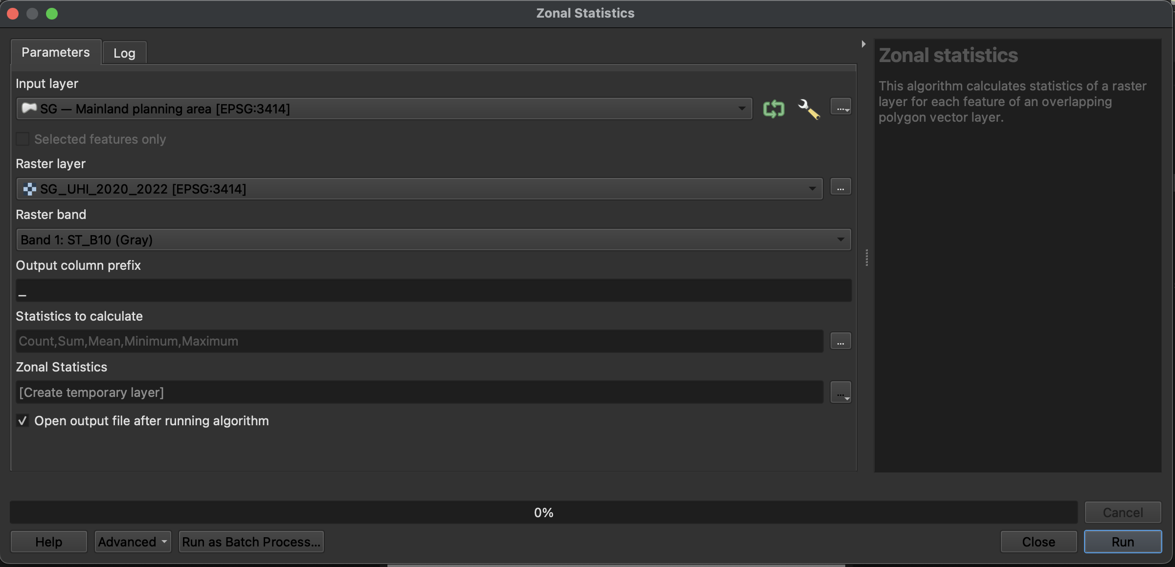
The average difference then can be calculated by first creating a relational join between the 2 different study periods where both the join field and target field are PLN_AREA_N respectively. The new average difference column then can be computed by calculating the difference between the 2 study periods.
Lastly the overall change in average temperature can be calculated by getting the sum of average LST difference by planning area divided by the total number of planning areas.